Recommender systems are one of the most successful and widely used applications of machine learning. Their use cases span a range of industries such as e-commerce, entertainment, and social media. As we showed in a previous post, RelationalAI’s knowledge graph coprocessor is a powerful tool for creating a social graph from an organization’s customer base. In this post, we will use the same RelationalAI Native App running on Snowpark Container Services within Snowflake’s Data Cloud to develop a fundamental and effective recommender system that falls under the umbrella of neighborhood-based recommender systems.

What are neighborhood-based recommender systems?

Neighborhood-based recommender systems belong to the category of collaborative filtering recommendation techniques. Within this framework, there are two main approaches: user-based and item-based systems.

User-based systems focus on behavioral patterns, such as movies that users have watched in the past, to identify similar users. Item-based systems focus on identifying items that draw similar interest from users. This blogpost will showcase how we can build an item-based recommender system, but note that the approach to build a user-based system is very similar.

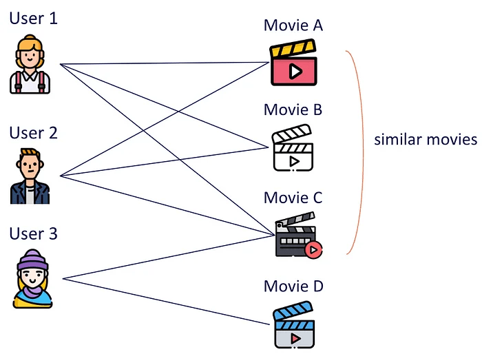
The below graph illustrates an example of the item-based method. Both users 1 and 2 have watched movies A and C, indicating that these movies appeal to similar audiences. So, we infer that movies A and C are similar. Based on this, we can suggest to user 3 that they watch movie A, given their interest in movie C.

Example of the item-based approach

Building a Movie Recommendation System

Let’s construct a movie recommendation system based on user-item interactions using the popular MovieLens100K dataset. Here’s an outline of the steps involved:

Step 1: We convert user-item interactions to a graph.
Step 2: We use user-item interactions to compute item-item similarities by leveraging similarity metrics provided by our graph analytics python library.
Step 3: We use the similarities computed in the previous step to predict the scores for all (user, movie) pairs. Each score is an indication of how likely it is for a user to watch the movie.
Step 4: We rank the scores for every user and generate recommendations.
Step 5: We evaluate the performance of the method using well known metrics.

The above steps can be seamlessly implemented using RelationalAI’s Native App running on Snowpark Container Services within Snowflake’s Data Cloud.

Step 1: Use user-item interactions to construct the graph

First we need to define some rules to describe objects in a model and the relationships between them. We will use the data in the Train (training set) object to populate the model. We first load information into User types and into Movie types and then we connect them based on the data in the training set.

# Define User Typewith model.rule(): t = Train() User.add(user_id=t.user_id)# Define Movie Typewith model.rule(): item = Items() train = Train() train.item_id == item.item_id Movie.add(item_id=train.item_id, title=item.title)# Link Users to Movieswith model.rule(): t = Train() u = User(user_id=t.user_id) m = Movie(item_id=t.item_id) u.watched.add(m)

Next, we use the RelationalAI object graph and attach our model to it by executing this one line of code:

movie_graph = Graph(model, undirected=True)

Then, we write a rule that takes all user objects and creates edges between them and movies they watched in our graph object. This will implicitly also add nodes.

# Add edges to the graph between users and movieswith model.rule(): u = User() movie_graph.Edge.add( u, u.watched )

Step 2: Compute Item-Item similarities

Now that we have modeled our data as a graph, we can compute item-item similarities using the user-item interactions: We want movies that have been watched by the same users to be more similar than movies that have not. We can do this by computing the cosine similarity between all pairs of movies.

with model.rule(): m1 = Movie() m2 = Movie() m1 != m2 # Compute cosine similarity between m1 and m2 similarity_score = movie_graph.compute.cosine_similarity(m1, m2) # Add objects to Similarity Type Similarity.add( movie1=Movie(item_id=m1.item_id), movie2=Movie(item_id=m2.item_id), similarity_score=similarity_score, )

Here’s an example of the top 5 movies similar to the popular Titanic movie based on cosine similarity scores:

Top 5 similar movies to Titanic

Step 3: Predicting scores for (user, movie) pairs

We then use the similarities calculated in the previous step to compute scores for all pairs of users and movies. This score captures the intuition that a user will watch movies that are similar to the movies they have watched in the past.

with model.rule(): u = User() m = Movie() # Top k similar movie detrmined by the similarity score n = NearestNeighbors() # Remove movies already watched by users from scoring with model.not_found(): m == u.watched # Find similar movies to movie m n.movie.item_id == m.item_id # Get intersection between watched movies and similar movies to m n.nearest_movies == u.watched # Calculate the sum similarity scores for each neighbor movie score_sum = aggregates.sum(n.similarity_score, per=[n.movie]) # Define Scoring type with user, movie, and score Scoring.add( user=u, movie=m, score=score_sum )

Step 4: Generating Top-k Recommendations

To generate a list of 10 recommendations (k=10) for each user, the last step is to rank the scores for the particular user and recommend the movies with the highest scores.

with model.rule(): s = Scoring() # Get top 10 movies based on the score score_rank = aggregates.top(10, s.score, s, per=[s.user]) Recommendation.add( user=s.user, score_rank = alias(score_rank, "score_rank"), recommended_movie = s.movie, score = s.score )

Step 5: Evaluating the item-based approach

To evaluate the performance of our method, we define a set of evaluation metrics that are widely used (such as precision and recall). These metrics compute how much our recommended items overlap with the true watched items of a given user that exists in a hidden test set.

Below is the code that implements average precision:

# Calculate Precision per Userwith model.rule(): u = User() r = Recommendation(user=u) # Count the number of recommended items that are relevant u.relevant == r.recommended_movie # Calculate precision for users true_positive = aggregates.count(u.relevant.item_id, per=[u.user_id]) user_precision = true_positive / k_recommendations # Add user_precision as an attribute u.set(user_precision=user_precision)# Get Average Precisionwith model.query() as select: u = User() u.relevant user_precision = u.user_precision.or_(0.0) total_precision = aggregates.avg(u, user_precision) precision = select( alias(total_precision, "Average Precision") )

Now we are able to serve recommendations to all of the customers in our database. For a value of K=10, the above recommendation system performs as well as others in the literature for neighborhood-based algorithms (average precision for this method with k=10 is 31.2%) while all customer data remains securely stored in snowflake.

Conclusion

Thanks to RelationalAI’s Native App on Snowflake, we built a recommendation system with just a few steps. Although the dataset used was a small graph with thousands of nodes and edges, our solution can scale to real world datasets due to our cloud-native architecture that separates compute from storage.

Utilizing cosine similarity for movie recommendations represents just one facet of the diverse spectrum of recommender systems available. In fact, the potential applications extend far beyond, limited only by the creativity of the practitioner. Venture into the realm of graph analytics and unlock a myriad of opportunities waiting to be explored!